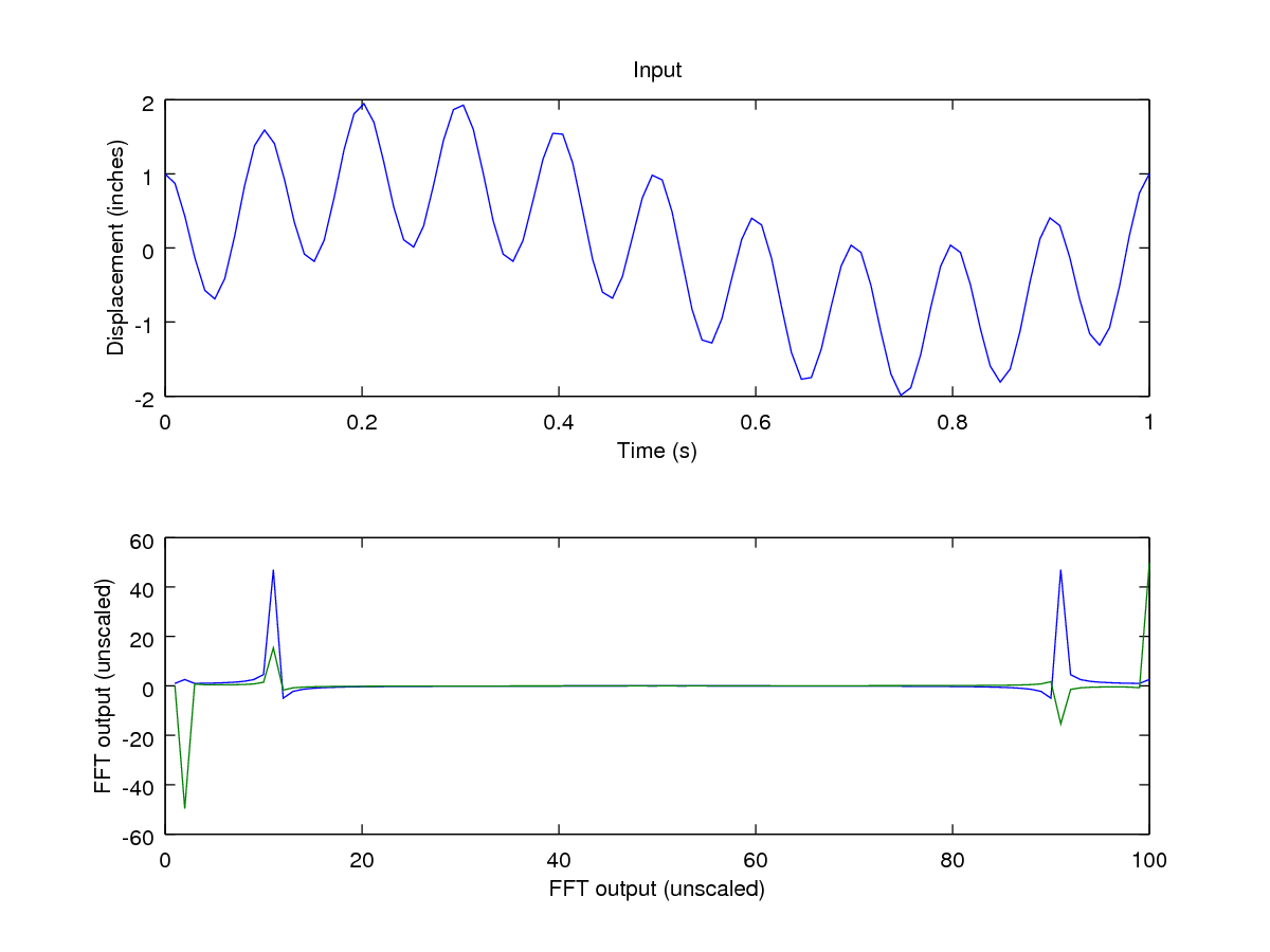
I use matlab almost exclusively for data processing. Matlab has many built-in functions that really make signal processing very quick and efficient. However, their FFT function is not one of them. Matlab's FFT is what I tend to think of as a ``mathematician's FFT''. It computes the basic transform exactly as written in the math textbooks. But what we are after is more of an ``engineer's FFT''. The main shortfalls of matlab's FFT function are:
|
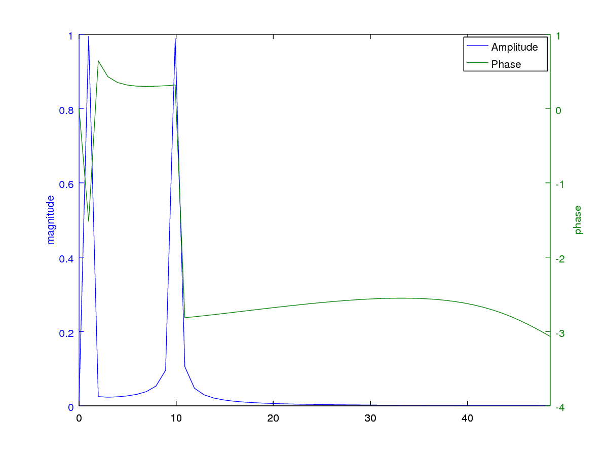
The function below is simple wrapper script that corrects all of these deficiencies and gives a proper ``engineer's FFT''. I recommend that you use a function like this all the time, and never use matlab's fft() directly. Note: this function does not do any windowing. This topic is discussed later in this section. The result of using this function is shown in 13. See how much more useful that is?
% Purpose: perform an FFT of a real-valued input signal, and generate the single-sided
% output, in amplitude and phase, scaled to the same units as the input.
%inputs:
% signal: the signal to transform
% ScanRate: the sampling frequency (in Hertz)
% outputs:
% frq: a vector of frequency points (in Hertz)
% amp: a vector of amplitudes (same units as the input signal)
% phase: a vector of phases (in radians)
function [frq, amp, phase] = simpleFFT( signal, ScanRate)
n = length(signal);
z = fft(signal, n); %do the actual work
%generate the vector of frequencies
halfn = floor(n / 2)+1;
deltaf = 1 / ( n / ScanRate);
frq = (0:(halfn-1)) * deltaf;
% convert from 2 sided spectrum to 1 sided
%(assuming that the input is a real signal)
amp(1) = abs(z(1)) ./ (n);
amp(2:(halfn-1)) = abs(z(2:(halfn-1))) ./ (n / 2);
amp(halfn) = abs(z(halfn)) ./ (n);
phase = angle(z(1:halfn));